In the beginning, there was data

Crestfallen by the seeming impossibility of recovering by beloved game from high school, I turned my attention to the original motivation: developing machine learning on the Apple ][+. Grabbing my manuals, I got to work.

Every solid machine learning project begins with data. My old clunker, however, is cut off from the world. I never had a modem but I recall one of my best friends using the modem on his Apple ][ to hack long distance access codes. (He since went on to pursue a successful career in telecommunications… naturally.) Even if I had a modem, what would I connect it to? Do those services still even exists? (I’m sure they do but I’m not going to figure that out today.) In the meantime, the plan is to create synthetic data locally.

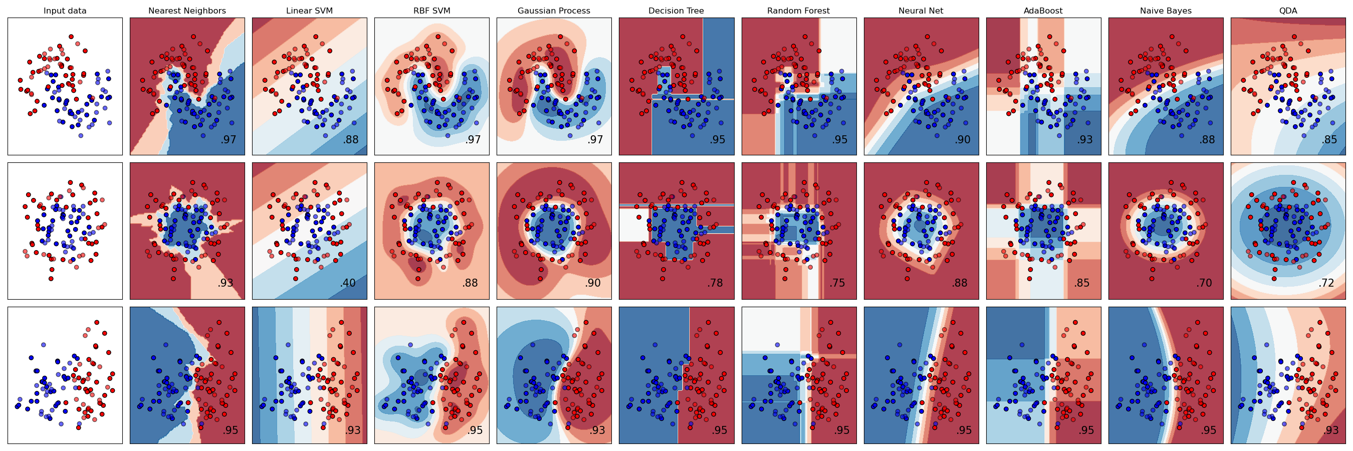
I’m sure everyone is familiar with the chart comparing different classification algorithms. Since two-dimensional binary classification seems like a great place to start, I’ll need a simple way to graph the data.

Fortunately, the Apple ][+ comes with a high-resolution graphics screen (HGR) that is 280 pixels across by 160 pixels high. (There is another mode with 192 vertical pixels but I wanted leave the bottom 4 lines of the text window visible for running output.) There are 8 color options for each pixel, but I have a green screen monitor, so I set everything to HCOLOR=7 (white2).

Drawing the axes

Deciding to stick to the positive quadrant, I wrote a subroutine (Applesoft BASIC does not have methods) to simply display the axes. Interestingly, coordinate (0,0) is the upper left corner of the screen while (279,159) is the lower right, so HPLOT 0,159 TO 279,159 draws the x-axis.

    500 REM  == SET GRAPHICS AND DRAW Y AXIS WITH TICK MARKS ==
    510 HGR : HCOLOR=7
    520 HPLOT 0,159 TO 279,159
    530 HPLOT 0,159 TO 0,0
    540 J = 0
    550 FOR I = 159 TO 0 STEP -10
    560   HPLOT 0,I TO 1,I
    570   IF J / 5 = INT(J / 5) THEN HPLOT 0,I TO 2,I
    580   IF J / 10 = INT(J / 10) THEN HPLOT 0,I TO 3,I
    590   J = J + 1
    600 NEXT I
    610 J = 0
    620 FOR I = 0 TO 279 STEP 10
    630   HPLOT I,159 TO I,158
    640   IF J / 5 = INT(J / 5) THEN HPLOT I,159 TO I,157
    650   IF J / 10 = INT(J / 10) THEN HPLOT I,159 TO I,156
    660   J = J + 1
    670 NEXT I
    680 RETURN

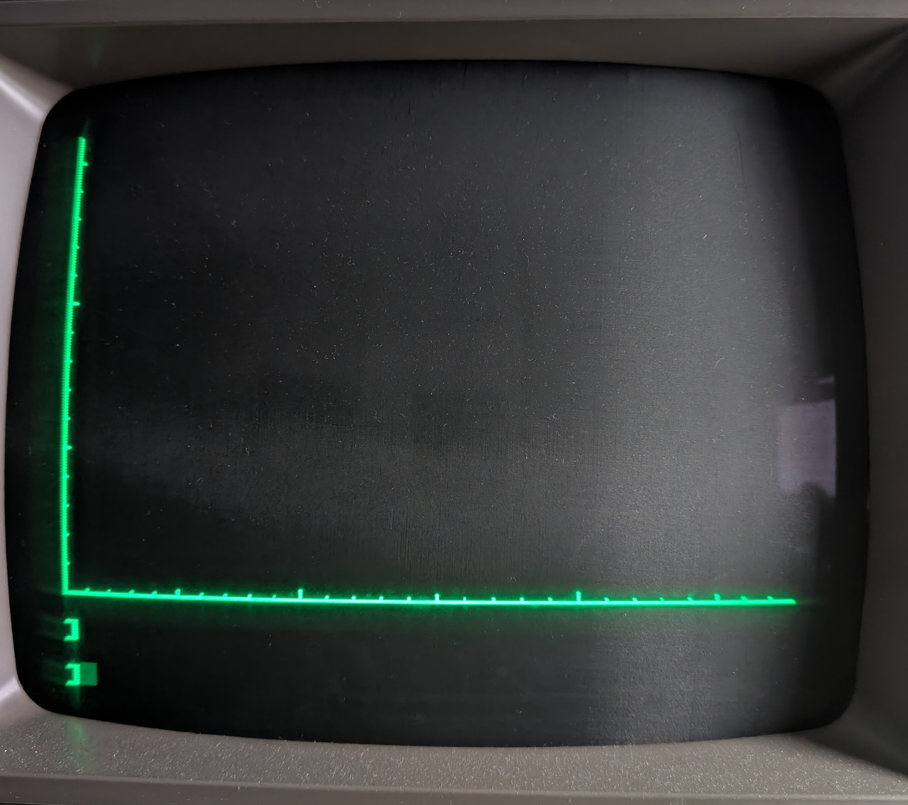
The first FOR I loop adds tick marks along the y-axis. I decided to get fancy and add elongated tick marks at every 5th unit and even longer ticks marks at every 10 unit. I use J to count the ticks. The second FOR I loop does the same for the x-axis. The final result looks like this:

Synthesizing the data

With a particular fondness for all thing Gaussian, I decided to create two sets of data points with Gaussian distributions. They look pretty and they’re fun.

    10  HOME : VTAB 21
    20  PI = 3.14159265
    30  GOSUB 500 : REM  DRAW AXIS
    40  DIM AM%(2) : REM  -- MEAN
    50  DIM BM%(2)
    60  DIM AS%(2) : REM  -- STD
    70  DIM BS%(2)
    80  REM  == HYPERPARAMETERS ==
    90  AN = 100 : REM  # OF POINTS
    100 BN = 50
    110 AM%(1) = 100 : AM%(2) = 50
    120 BM%(1) = 200 : BM%(2) = 100
    130 AS%(1) = 30 : AS%(2) = 10
    140 BS%(1) = 50 : BS%(2) = 25
    150 AC = 0.5
    160 BC = -0.5
    170 REM  == END HYPERPARAMETERS ==

HOME clears the screen and VTAB 21 moves the cursor to the 21st text line on the screen, which will be the first line under the graphics after HGR. The Apple ][+ doesn’t come with a constant for π so I set that up using all the precision available.

AM% is a two element array of integers to store, respectively, the x-mean and y-mean values for the A data set. (The % sign makes the variable an integer which save space but actually reduced performance because mathematical operations on the Apple ][+ convert integers to real numbers and then back again.) AS% does the same for the x- and y-standard deviations. AC is a real number correlation coefficient ∈ [-1, 1]. Finally, AN is the number of elements in the A dataset. The corresponding B data set hyperparameters are similar. (In Applesoft BASIC only the first two characters of a variable name are ‘considered’ so you have to be careful of collisions.)

Box-Muller to the rescue

The Apple ][+ can generate uniform random variables from 0 to 0.999999999 using RND(), however, to get standard normal random variables we’ll have to use the Box-Muller transform.

Given two independent samples, \(u_1\) and \(u_2\), chosen from a uniform distribution on the unit interval (0, 1), we can get two independent random variables, \(z_0\) and \(z_1\), with a standard normal distribution with the following:

\[z_0 = R \cos(\theta) = \sqrt{-2 \ln(u_1)} \cos(2 \pi u_2) \\ z_1 = R \sin(\theta) = \sqrt{-2 \ln(u_1)} \sin(2 \pi u_2)\]

Here is the code to do that.

900 REM  == BOX-MULLER TRANSFORM ==
910 U1 = RND(1)
920 U2 = RND(1)
930 R = SQR(-2 * LOG(U1))
940 TH = 2 * PI * U2
950 Z0 = R * COS(TH)
960 Z1 = R * SIN(TH)
970 RETURN

From there, to obtain a 2D Gaussian with mean \(\mu_x, \mu_y\) and covariance matrix \(\Sigma\), we’ll need to apply the following, where \(\sigma_x\) and \(\sigma_y\) are the standard deviations in the \(x\) and \(y\) directions, and \(\rho\) is the correlation coefficient:

\[x = \mu_x + \sigma_x z_1 \\ y = \mu_y + \rho \sigma_y z_1 + \sqrt{1 - \rho^2} \sigma_y z_2\]

Here is the code that generates all the samples using these transformations.

200 DIM AX%(AN,2)
210 DIM BX%(BN,2)
220 FOR I = 1 TO AN
230   GOSUB 900 : REM FETCH STANDARD NORMAL RANDOM VALUES
240   X% = AM%(1) + AS%(1) * Z0
250   Y% = AM%(2) + AC * AS%(2) * Z0 + SQR(1 - AC ^ 2) * AS%(2) * Z1
260   AX%(I,1) = X%
270   AX%(I,2) = Y%
280   PRINT "POINT IN SET A "; I; " AT ("; X%; ","; Y%; ")"
290   GOSUB 700 : REM  DRAW A +
300 NEXT I
310 FOR I = 1 TO BN
320   GOSUB 900 : REM FETCH STANDARD NORMAL RANDOM VALUES
330   X% = BM%(1) + BS%(1) * Z0
340   Y% = BM%(2) + BC * BS%(2) * Z0 + SQR(1 - BC ^ 2) * BS%(2) * Z1
350   BX%(I,1) = X%
360   BX%(I,2) = Y%
370   PRINT "POINT IN SET B "; I; " AT ("; X%; ","; Y%; ")"
380   GOSUB 800 : REM  DRAW A BOX
390 NEXT I
400 END

I decided to store the data samples in AX% and BX% as integers to save on memory. Since they are all randomly generated, the extra precision won’t make much of a difference anyway. I’m using 2D arrays where the first axis is the number of samples (e.g., AN) and the second axis is the feature dimension (e.g., 2 for \(x\) and \(y\)).

You can see calling GOSUB 700 and GOSUB 800 to plot the points. Here is the final code for that.

700 REM == DRAW + AT X,Y ==
710 IF X% < 1 OR X% > 270 THEN RETURN
720 IF Y% < 1 OR Y% > 150 THEN RETURN
730 HPLOT X% - 1,Y% TO X% + 1,Y%
740 HPLOT X%,Y% - 1 TO X%,Y% + 1
750 RETURN
800 REM == DRAW BOX AT X,Y ==
810 IF X% < 1 OR X% > 270 THEN RETURN
820 IF Y% < 1 OR Y% > 150 THEN RETURN
830 HPLOT X% - 1,Y% - 1 TO X% + 1,Y% - 1
840 HPLOT X% - 1,Y%: HPLOT X% + 1,Y%
850 HPLOT X% - 1,Y% + 1 TO X% + 1,Y% + 1
860 RETURN

I first verify that the data point is on the visible region of the graph (plotting off the screen will throw an error) and then draw either a “+” or a “□”.

Running the code

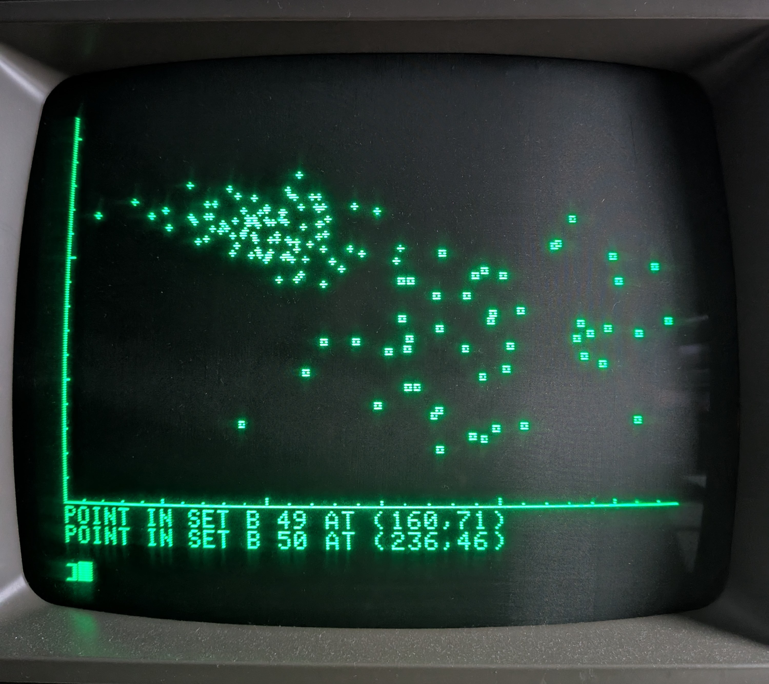
Putting it all together, it takes the Apple ][+ about a minute to generate and plot 150 data points. The end result looks like this.

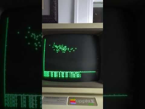
Watch this video if you’d like to see it run, in all it’s glory.

Now that this is out of the way, we’ll start by implementing one of the simplest and easiest to understand machine learning algorithms.